Built-in Modeling Language

Gen provides a built-in embedded modeling language for defining generative functions. The language uses a syntax that extends Julia's syntax for defining regular Julia functions, and is also referred to as the Dynamic Modeling Language.

Generative functions in the modeling language are identified using the @gen keyword in front of a Julia function definition. Here is an example @gen function that samples two random choices:

@gen function foo(prob::Float64=0.1)
    z1 = @trace(bernoulli(prob), :a)
    z2 = @trace(bernoulli(prob), :b)
    return z1 || z2
end

After running this code, foo is a Julia value of type DynamicDSLFunction:

Gen.DynamicDSLFunction — Type

DynamicDSLFunction{T} <: GenerativeFunction{T,DynamicDSLTrace}

A generative function based on a shallowly embedding modeling language based on Julia functions.

Constructed using the @gen keyword. Most methods in the generative function interface involve a end-to-end execution of the function.

source

Note that it is possible to provide default values for trailing positional arguments. However, keyword arguments are currently not supported.

We can call the resulting generative function like we would a regular Julia function:

retval::Bool = foo(0.5)

We can also trace its execution:

(trace, _) = generate(foo, (0.5,))

Optional arguments can be left out of the above operations, and default values will be filled in automatically:

julia> (trace, _) = generate(foo, (,));
julia> get_args(trace)
(0.1,)

See Generative Functions for the full set of operations supported by a generative function. Note that the built-in modeling language described in this section is only one of many ways of defining a generative function – generative functions can also be constructed using other embedded languages, or by directly implementing the methods of the generative function interface. However, the built-in modeling language is intended to being flexible enough cover a wide range of use cases. In the remainder of this section, we refer to generative functions defined using the built-in modeling language as @gen functions. Details about the implementation of @gen functions can be found in the Modeling Language Implementation section.

Annotations

Annotations are a syntactic construct in the built-in modeling language that allows users to provide additional information about how @gen functions should be interpreted. Annotations are optional, and not necessary to understand the basics of Gen. There are two types of annotations – argument annotations and function annotations.

Argument annotations. In addition to type declarations on arguments like regular Julia functions, @gen functions also support additional annotations on arguments. Each argument can have the following different syntactic forms:

y: No type declaration; no annotations.
y::Float64: Type declaration; but no annotations.
(grad)(y): No type declaration provided;, annotated with grad.
(grad)(y::Float64): Type declaration provided; and annotated with grad.

Currently, the possible argument annotations are:

grad (see Differentiable programming).

Function annotations. The @gen function itself can also be optionally associated with zero or more annotations, which are separate from the per-argument annotations. Function-level annotations use the following different syntactic forms:

@gen function foo(<args>) <body> end: No function annotations.
@gen (grad) function foo(<args>) <body> end: The function has the grad annotation.
@gen (grad,static) function foo(<args>) <body> end: The function has both the grad and static annotations.

Currently the possible function annotations are:

grad (see Differentiable programming).
static (see Static Modeling Language).
nojuliacache (see Static Modeling Language).

Making random choices

Random choices are made by calling a probability distribution on some arguments:

val::Bool = bernoulli(0.5)

See Probability Distributions for the set of built-in probability distributions, and for information on implementing new probability distributions.

In the body of a @gen function, wrapping a call to a random choice with an @trace expression associates the random choice with an address, and evaluates to the value of the random choice. The syntax is:

@trace(<distribution>(<args>), <addr>)

Addresses can be any Julia value. Here, we give the Julia symbol address :z to a Bernoulli random choice.

val::Bool = @trace(bernoulli(0.5), :z)

Not all random choices need to be given addresses. An address is required if the random choice will be observed, or will be referenced by a custom inference algorithm (e.g. if it will be proposed to by a custom proposal distribution).

Sample space and support of random choices

Different probability distributions produce different types of values for their random choices. For example, the bernoulli distribution results in Bool values (either true or false), the normal distribution results in Real values that may be positive or negative, and the beta distribution result in Real values that are always in the unit interval (0, 1).

Each Distribution is associated with two sets of values:

The sample space of the distribution, which does not depend on the arguments.
The support of the distribution, which may depend on the arguments, and is the set of values that has nonzero probability (or probability density). It may be the entire sample space, or it may be a subset of the sample space.

For example, the sample space of bernoulli is Bool and its support is either {true}, {false}, or {true, false}. The sample space of normal is Real and its support is the set of all values on the real line. The sample space of beta is Real and its support is the set of values in the interval (0, 1).

Gen's built in modeling languages require that a address is associated with a fixed sample space. For example, it is not permitted to use a bernoulli distribution to sample at addresss :a in one execution, and a normal distribution to sample at address :a in a different execution, because their sample spaces differ (Bool vs Real):

@gen function foo()
    if @trace(bernoulli(0.5), :branch)
        @trace(bernoulli(0.5), :x)
    else
        @trace(normal(0, 1), :x)
    end
end

A generative function can be disciplined or not. In a disciplined generative function, the support of random choices at each address must be fixed. That is, for each address a there must exist a set S that is a subset of the sample space such that for all executions of the generative function, if a occurs as the address of a choice in the execution, then the support of that choice is exactly S. Violating this discipline will cause NaNs, errors, or undefined behavior in some inference programs. However, in many cases it is convenient to write an inference program that operates correctly and efficiently on some specialized class of undisciplined models. In these cases, authors who want their inference code to be reusable should consider documenting which kinds of undisciplined models their inference algorithms allow or expect to see.

If the support of a random choice needs to change, a disciplined generative function can represent this by using a different address for each distinct value of the support. For example, consider the following generative function:

@gen function foo()
    n = @trace(categorical([0.5, 0.5]), :n) + 1
    @trace(categorical(ones(n) / n), :x)
end

The support of the random choice with address :x is either the set $\{1, 2\}$ or $\{1, 2, 3\}$. Therefore, this random choice does not have constant support, and the generative function foo is not 'disciplined'. Specifically, this could result in undefined behavior for the following inference program:

tr, _ = importance_resampling(foo, (), choicemap((:x, 3)))

It is recommended to write disciplined generative functions when possible.

Calling generative functions

@gen functions can invoke other generative functions in three ways:

Untraced call: If foo is a generative function, we can invoke foo from within the body of a @gen function using regular call syntax. The random choices made within the call are not given addresses in our trace, and are therefore untraced random choices (see Generative Function Interface for details on untraced random choices).

val = foo(0.5)

Traced call with a nested address namespace: We can include the traced random choices made by foo in the caller's trace, under a namespace, using @trace:

val = @trace(foo(0.5), :x)

Now, all random choices made by foo are included in our trace, under the namespace :x. For example, if foo makes random choices at addresses :a and :b, these choices will have addresses :x => :a and :x => :b in the caller's trace.

Traced call with shared address namespace: We can include the traced random choices made by foo in the caller's trace using @trace:

val = @trace(foo(0.5))

Now, all random choices made by foo are included in our trace. The caller must guarantee that there are no address collisions. NOTE: This type of call can only be used when calling other @gen functions. Other types of generative functions cannot be called in this way.

Composite addresses

In Julia, Pair values can be constructed using the => operator. For example, :a => :b is equivalent to Pair(:a, :b) and :a => :b => :c is equivalent to Pair(:a, Pair(:b, :c)). A Pair value (e.g. :a => :b => :c) can be passed as the address field in an @trace expression, provided that there is not also a random choice or generative function called with @trace at any prefix of the address.

Consider the following examples.

This example is invalid because :a => :b is a prefix of :a => :b => :c:

@trace(normal(0, 1), :a => :b => :c)
@trace(normal(0, 1), :a => :b)

This example is invalid because :a is a prefix of :a => :b => :c:

@trace(normal(0, 1), :a => :b => :c)
@trace(normal(0, 1), :a)

This example is invalid because :a => :b is a prefix of :a => :b => :c:

@trace(normal(0, 1), :a => :b => :c)
@trace(foo(0.5), :a => :b)

This example is invalid because :a is a prefix of :a => :b:

@trace(normal(0, 1), :a)
@trace(foo(0.5), :a => :b)

This example is valid because :a => :b and :a => :c are not prefixes of one another:

@trace(normal(0, 1), :a => :b)
@trace(normal(0, 1), :a => :c)

This example is valid because :a => :b and :a => :c are not prefixes of one another:

@trace(normal(0, 1), :a => :b)
@trace(foo(0.5), :a => :c)

Tilde syntax

As a short-hand for @trace expressions, the tilde operator ~ can also be used to make random choices and traced calls to generative functions. For example, the expression

{:x} ~ normal(0, 1)

is equivalent to:

@trace(normal(0, 1), :x)

One can also conveniently assign random values to variables using the syntax:

x ~ normal(0, 1)

which is equivalent to:

x = @trace(normal(0, 1), :x)

Finally, one can make traced calls using a shared address namespace with the syntax:

{*} ~ foo(0.5)

which is equivalent to:

@trace(foo(0.5))

Note that ~ is also defined in Base as a unary operator that performs the bitwise-not operation (see Base.:~). This use of ~ is also supported within @gen functions. However, uses of ~ as a binary infix operator within an @gen function will always be treated as equivalent to an @trace expression. If your module contains its own two-argument definition YourModule.:~(a, b) of the ~ function, calls to that function within @gen functions have to be in qualified prefix form, i.e., you have to write YourModule.:~(a, b) instead of a ~ b.

Return value

Like regular Julia functions, @gen functions return either the expression used in a return keyword, or by evaluating the last expression in the function body. Note that the return value of a @gen function is different from a trace of @gen function, which contains the return value associated with an execution as well as the assignment to each random choice made during the execution. See Generative Function Interface for more information about traces.

Trainable parameters

A @gen function may begin with an optional block of trainable parameter declarations. The block consists of a sequence of statements, beginning with @param, that declare the name and Julia type for each trainable parameter. The function below has a single trainable parameter theta with type Float64:

@gen function foo(prob::Float64)
    @param theta::Float64
    z1 = @trace(bernoulli(prob), :a)
    z2 = @trace(bernoulli(theta), :b)
    return z1 || z2
end

Trainable parameters obey the same scoping rules as Julia local variables defined at the beginning of the function body. The value of a trainable parameter is undefined until it is initialized using init_param!. In addition to the current value, each trainable parameter has a current gradient accumulator value. The gradient accumulator value has the same shape (e.g. array dimension) as the parameter value. It is initialized to all zeros, and is incremented by accumulate_param_gradients!.

The following methods are exported for the trainable parameters of @gen functions:

Gen.init_param! — Function

init_param!(gen_fn::Union{DynamicDSLFunction,StaticIRGenerativeFunction}, name::Symbol, value)

Initialize the the value of a named trainable parameter of a generative function.

Also generates the gradient accumulator for that parameter to zero(value).

Example:

init_param!(foo, :theta, 0.6)

source

Gen.get_param — Function

value = get_param(gen_fn::Union{DynamicDSLFunction,StaticIRGenerativeFunction}, name::Symbol)

Get the current value of a trainable parameter of the generative function.

source

Gen.get_param_grad — Function

value = get_param_grad(gen_fn::Union{DynamicDSLFunction,StaticIRGenerativeFunction}, name::Symbol)

Get the current value of the gradient accumulator for a trainable parameter of the generative function.

source

Gen.set_param! — Function

set_param!(gen_fn::Union{DynamicDSLFunction,StaticIRGenerativeFunction}, name::Symbol, value)

Set the value of a trainable parameter of the generative function.

NOTE: Does not update the gradient accumulator value.

source

Gen.zero_param_grad! — Function

zero_param_grad!(gen_fn::Union{DynamicDSLFunction,StaticIRGenerativeFunction}, name::Symbol)

Reset the gradient accumlator for a trainable parameter of the generative function to all zeros.

source

Trainable parameters are designed to be trained using gradient-based methods. This is discussed in the next section.

Differentiable programming

Given a trace of a @gen function, Gen supports automatic differentiation of the log probability (density) of all of the random choices made in the trace with respect to the following types of inputs:

all or a subset of the arguments to the function.
the values of all or a subset of random choices.
all or a subset of trainable parameters of the @gen function.

We first discuss the semantics of these gradient computations, and then discuss what how to write and use Julia code in the body of a @gen function so that it can be automatically differentiated by the gradient computation.

Supported gradient computations

Gradients with respect to arguments. A @gen function may have a fixed set of its arguments annotated with grad, which indicates that gradients with respect to that argument should be supported. For example, in the function below, we indicate that we want to support differentiation with respect to the y argument, but that we do not want to support differentiation with respect to the x argument.

@gen function foo(x, (grad)(y))
    if x > 5
        @trace(normal(y, 1), :z)
    else
        @trace(normal(y, 10), :z)
    end
end

For the function foo above, when x > 5, the gradient with respect to y is the gradient of the log probability density of a normal distribution with standard deviation 1, with respect to its mean, evaluated at mean y. When x <= 5, we instead differentiate the log density of a normal distribution with standard deviation 10, relative to its mean.

Gradients with respect to values of random choices. The author of a @gen function also identifies a set of addresses of random choices with respect to which they wish to support gradients of the log probability (density). Gradients of the log probability (density) with respect to the values of random choices are used in gradient-based numerical optimization of random choices, as well as certain MCMC updates that require gradient information.

Gradients with respect to trainable parameters. The gradient of the log probability (density) with respect to the trainable parameters can also be computed using automatic differentiation. Currently, the log probability (density) must be a differentiable function of all trainable parameters.

Gradients of a function of the return value. Differentiable programming in Gen composes across function calls. If the return value of the @gen function is conditionally dependent on source elements including (i) any arguments annotated with grad or (ii) any random choices for which gradients are supported, or (ii) any trainable parameters, then the gradient computation requires a gradient of the an external function with respect to the return value in order to the compute the correct gradients. Thus, the function being differentiated always includes a term representing the log probability (density) of all random choices made by the function, but can be extended with a term that depends on the return value of the function. The author of a @gen function can indicate that the return value depends on the source elements (causing the gradient with respect to the return value is required for all gradient computations) by adding the grad annotation to the @gen function itself. For example, in the function below, the return value is conditionally dependent (and actually identical to) on the random value at address :z:

@gen function foo(x, (grad)(y))
    if x > 5
        return @trace(normal(y, 1), :z)
    else
        return @trace(normal(y, 10), :z)
    end
end

If the author of foo wished to support the computation of gradients with respect to the value of :z, they would need to add the grad annotation to foo using the following syntax:

@gen (grad) function foo(x, (grad)(y))
    if x > 5
        return @trace(normal(y, 1), :z)
    else
        return @trace(normal(y, 10), :z)
    end
end

Writing differentiable code

In order to compute the gradients described above, the code in the body of the @gen function needs to be differentiable. Code in the body of a @gen function consists of:

Julia code
Making random choices
Calling generative functions

We now discuss how to ensure that code of each of these forms is differentiable. Note that the procedures for differentiation of code described below are only performed during certain operations on @gen functions (choice_gradients and accumulate_param_gradients!).

Julia code. Julia code used within a body of a @gen function is made differentiable using the ReverseDiff package, which implements reverse-mode automatic differentiation. Specifically, values whose gradient is required (either values of arguments, random choices, or trainable parameters) are 'tracked' by boxing them into special values and storing the tracked value on a 'tape'. For example a Float64 value is boxed into a ReverseDiff.TrackedReal value. Methods (including e.g. arithmetic operators) are defined that operate on these tracked values and produce other tracked values as a result. As the computation proceeds all the values are placed onto the tape, with back-references to the parent operation and operands. Arithmetic operators, array and linear algebra functions, and common special numerical functions, as well as broadcasting, are automatically supported. See ReverseDiff for more details.

Making random choices. When making a random choice, each argument is either a tracked value or not. If the argument is a tracked value, then the probability distribution must support differentiation of the log probability (density) with respect to that argument. Otherwise, an error is thrown. The has_argument_grads function indicates which arguments support differentiation for a given distribution (see Probability Distributions). If the gradient is required for the value of a random choice, the distribution must support differentiation of the log probability (density) with respect to the value. This is indicated by the has_output_grad function.

Calling generative functions. Like distributions, generative functions indicate which of their arguments support differentiation, using the has_argument_grads function. It is an error if a tracked value is passed as an argument of a generative function, when differentiation is not supported by the generative function for that argument. If a generative function gen_fn has accepts_output_grad(gen_fn) = true, then the return value of the generative function call will be tracked and will propagate further through the caller @gen function's computation.

Static Modeling Language

The static modeling language is a restricted variant of the built-in modeling language. Models written in the static modeling language can result in better inference performance (more inference operations per second and less memory consumption), than the full built-in modeling language, especially for models used with iterative inference algorithms like Markov chain Monte Carlo.

A function is identified as using the static modeling language by adding the static annotation to the function. For example:

@gen (static) function foo(prob::Float64)
    z1 = @trace(bernoulli(prob), :a)
    z2 = @trace(bernoulli(prob), :b)
    z3 = z1 || z2
    z4 = !z3
    return z4
end

After running this code, foo is a Julia value whose type is a subtype of StaticIRGenerativeFunction, which is a subtype of GenerativeFunction.

Static computation graph

Using the static annotation instructs Gen to statically construct a directed acyclic graph for the computation represented by the body of the function. For the function foo above, the static graph looks like:

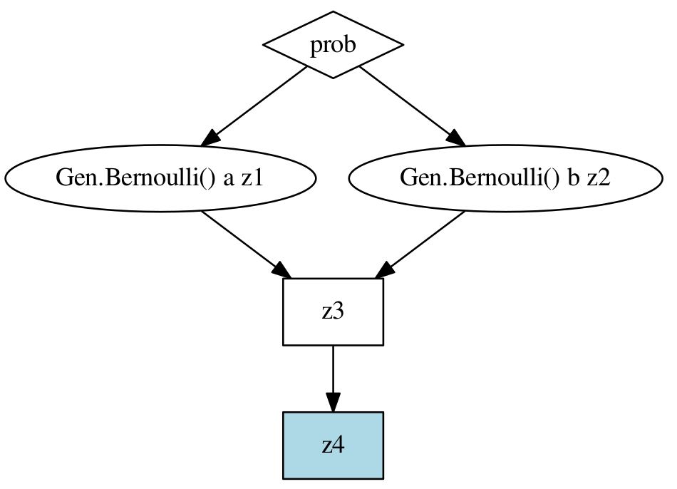
In this graph, oval nodes represent random choices, square nodes represent Julia computations, and diamond nodes represent arguments. The light blue shaded node is the return value of the function. Having access to the static graph allows Gen to generate specialized code for Updating traces that skips unecessary parts of the computation. Specifically, when applying an update operation, the graph is analyzed, and each value in the graph identified as having possibly changed, or not. Nodes in the graph do not need to be re-executed if none of their input values could have possibly changed. Also, even if some inputs to a generative function node may have changed, knowledge that some of the inputs have not changed often allows the generative function being called to more efficiently perform its update operation. This is the case for functions produced by Generative Function Combinators.

You can plot the graph for a function with the static annotation if you have PyCall installed, and a Python environment that contains the graphviz Python package, using, e.g.:

using PyCall
@pyimport graphviz
using Gen: draw_graph
draw_graph(foo, graphviz, "test")

This will produce a file test.pdf in the current working directory containing the rendered graph.

Restrictions

First, the definition of a (static) generative function is always expected to occur as a top-level definition (aka global variable); usage in non–top-level scopes is unsupported and may result in incorrect behavior.

Next, in order to be able to construct the static graph, Gen restricts the permitted syntax that can be used in functions annotated with static. In particular, each statement in the body must be one of the following:

A @param statement specifying any Trainable parameters, e.g.:

@param theta::Float64

An assignment, with a symbol or tuple of symbols on the left-hand side, and a Julia expression on the right-hand side, which may include @trace expressions, e.g.:

mu, sigma = @trace(bernoulli(p), :x) ? (mu1, sigma1) : (mu2, sigma2)

A top-level @trace expression, e.g.:

@trace(bernoulli(1-prob_tails), :flip)

All @trace expressions must use a literal Julia symbol for the first component in the address. Unlike the full built-in modeling-language, the address is not optional.

A return statement, with a Julia expression on the right-hand side, e.g.:

return @trace(geometric(prob), :n_flips) + 1

The functions are also subject to the following restrictions:

Default argument values are not supported.
Constructing named or anonymous Julia functions (and closures) is not allowed.
List comprehensions with internal @trace calls are not allowed.
Splatting within @trace calls is not supported
Generative functions that are passed in as arguments cannot be traced.
For composite addresses (e.g. :a => 2 => :c) the first component of the address must be a literal symbol, and there may only be one statement in the function body that uses this symbol for the first component of its address.
Julia control flow constructs (e.g. if, for, while) cannot be used as top-level statements in the function body. Control flow should be implemented inside either Julia functions that are called, or other generative functions.

Certain loop constructs can be implemented using Generative Function Combinators instead. For example, the following loop:

for (i, prob) in enumerate(probs)
    @trace(foo(prob), :foo => i)
end

can instead be implemented as:

@trace(Map(foo)(probs), :foo)

Loading generated functions

Once a (static) generative function is defined, it can be used in the same way as a non-static generative function. In previous versions of Gen, the @load_generated_functions macro had to be called before a function with a (static) annotation could be used. This macro is no longer necessary, and will be removed in a future release.

Performance tips

For better performance when the arguments are simple data types like Float64, annotate the arguments with the concrete type. This permits a more optimized trace data structure to be generated for the generative function.

Caching Julia values

By default, the values of Julia computations (all calls that are not random choices or calls to generative functions) are cached as part of the trace, so that Updating traces can avoid unecessary re-execution of Julia code. However, this cache may grow the memory footprint of a trace. To disable caching of Julia values, use the function annotation nojuliacache (this annotation is ignored unless the static function annotation is also used).