Tutorial: Basics of Iterative Inference Programming in Gen

This tutorial introduces the basics of inference programming in Gen. In particular, in this notebook we’ll focus on iterative inference programs, which include Markov chain Monte Carlo algorithms.

The task: curve-fitting with outliers

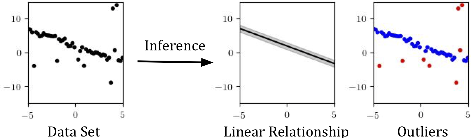
Suppose we have a dataset of points in the $x,y$ plane that is mostly explained by a linear relationship, but which also has several outliers. Our goal will be to automatically identify the outliers, and to find a linear relationship (a slope and intercept, as well as an inherent noise level) that explains rest of the points:

See https://dspace.mit.edu/bitstream/handle/1721.1/119255/MIT-CSAIL-TR-2018-020.pdf, Figure 2(a))

This is a simple inference problem. But it has two features that make it ideal for introducing concepts in modeling and inference.

First, we want not only to estimate the slope and intercept of the line that best fits the data, but also to classify each point as an inlier or outlier; that is, there are a large number of latent variables of interest, enough to make importance sampling an unreliable method (absent a more involved custom proposal that does the heavy lifting).
Second, several of the parameters we’re estimating (the slope and intercept) are continuous and amenable to gradient-based search techniques, which will allow us to explore Gen’s optimization capabilities.

Let’s get started!

Outline

Section 1. Writing the model: a first attempt

Section 2. Visualizing the model’s behavior

Section 3. The problem with generic importance sampling

Section 4. MCMC Inference Part 1: Block Resimulation

Section 5. MCMC Inference Part 2: Gaussian Drift

Section 6. MCMC Inference Part 3: Proposals based on heuristics

Section 7. MAP Optimization

import Random, Logging
using Gen, Plots

# Disable logging, because @animate is verbose otherwise
Logging.disable_logging(Logging.Info);

1. Writing the model

We begin, as usual, by writing a model: a generative function responsible (conceptually) for simulating a synthetic dataset.

Our model will take as input a vector of x coordinates, and produce as output corresponding y coordinates.

We will also use this opportunity to introduce some syntactic sugar. As described in the previous notebook, random choices in Gen are given addresses using the syntax {addr} ~ distribution(...). But this can be a bit verbose, and often leads to code that looks like the following:

x = {:x} ~ normal(0, 1)
slope = {:slope} ~ normal(0, 1)

In these examples, the variable name is duplicated as the address of the random choice. Because this is a common pattern, Gen provides syntactic sugar that makes it nicer to use:

# Desugars to "x = {:x} ~ normal(0, 1)"
x ~ normal(0, 1)
# Desugars to "slope = {:slope} ~ normal(0, 1)"
slope ~ normal(0, 1)

Note that sometimes, it is still necessary to use the {...} form, for example in loops:

# INVALID:
for i=1:10
    y ~ normal(0, 1) # The name :y will be used more than once!!
    println(y)
end

# VALID:
for i=1:10
    y = {(:y, i)} ~ normal(0, 1) # OK: the address is different each time.
    println(y)
end

We’ll use this new syntax for writing our model of linear regression with outliers. As we’ve seen before, the model generates parameters from a prior, and then simulates data based on those parameters:

@gen function regression_with_outliers(xs::Vector{<:Real})
    # First, generate some parameters of the model. We make these
    # random choices, because later, we will want to infer them
    # from data. The distributions we use here express our assumptions
    # about the parameters: we think the slope and intercept won't be
    # too far from 0; that the noise is relatively small; and that
    # the proportion of the dataset that don't fit a linear relationship
    # (outliers) could be anything between 0 and 1.
    slope ~ normal(0, 2)
    intercept ~ normal(0, 2)
    noise ~ gamma(1, 1)
    prob_outlier ~ uniform(0, 1)
    
    # Next, we generate the actual y coordinates.
    n = length(xs)
    ys = Float64[]
    
    for i = 1:n
        # Decide whether this point is an outlier, and set
        # mean and standard deviation accordingly
        if ({:data => i => :is_outlier} ~ bernoulli(prob_outlier))
            (mu, std) = (0., 10.)
        else
            (mu, std) = (xs[i] * slope + intercept, noise)
        end
        # Sample a y value for this point
        push!(ys, {:data => i => :y} ~ normal(mu, std))
    end
    ys
end;

2. What our model is doing: visualizing the prior

Let’s visualize what our model is doing by drawing some samples from the prior.

# Generate nine traces and visualize them
include("visualization/regression_viz.jl")
xs     = collect(range(-5, stop=5, length=20))
traces = [Gen.simulate(regression_with_outliers, (xs,)) for i in 1:9];
Plots.plot([visualize_trace(t) for t in traces]...)

svg

Legend:

red points: outliers;
blue points: inliers (i.e. regular data);
dark grey shading: noise associated with inliers; and
light grey shading: noise associated with outliers.

Note that an outlier can occur anywhere — including close to the line — and that our model is capable of generating datasets in which the vast majority of points are outliers.

3. The problem with generic importance sampling

To motivate the need for more complex inference algorithms, let’s begin by using the simple importance sampling method from the previous tutorial, and thinking about where it fails.

First, let us create a synthetic dataset to do inference about.

function make_synthetic_dataset(n)
    Random.seed!(1)
    prob_outlier = 0.2
    true_inlier_noise = 0.5
    true_outlier_noise = 5.0
    true_slope = -1
    true_intercept = 2
    xs = collect(range(-5, stop=5, length=n))
    ys = Float64[]
    for (i, x) in enumerate(xs)
        if rand() < prob_outlier
            y = randn() * true_outlier_noise
        else
            y = true_slope * x + true_intercept + randn() * true_inlier_noise
        end
        push!(ys, y)
    end
    (xs, ys)
end
    
(xs, ys) = make_synthetic_dataset(20);
Plots.scatter(xs, ys, color="black", xlabel="X", ylabel="Y", 
              label=nothing, title="Observations - regular data and outliers")

svg

We will to express our observations as a ChoiceMap that constrains the values of certain random choices to equal their observed values. Here, we want to constrain the values of the choices with address :data => i => :y (that is, the sampled $y$ coordinates) to equal the observed $y$ values. Let’s write a helper function that takes in a vector of $y$ values and creates a ChoiceMap that we can use to constrain our model:

function make_constraints(ys::Vector{Float64})
    constraints = Gen.choicemap()
    for i=1:length(ys)
        constraints[:data => i => :y] = ys[i]
    end
    constraints
end;

We can apply it to our dataset’s vector of ys to make a set of constraints for doing inference:

observations = make_constraints(ys);

Now, we use the library function importance_resampling to draw approximate posterior samples given those observations:

function logmeanexp(scores)
    logsumexp(scores) - log(length(scores))
end;

traces    = [first(Gen.importance_resampling(regression_with_outliers, (xs,), observations, 2000)) for i in 1:9]
log_probs = [get_score(t) for t in traces]
println("Average log probability: $(logmeanexp(log_probs))")
Plots.plot([visualize_trace(t) for t in traces]...)

Average log probability: -51.8570956904098

svg

We see here that importance resampling hasn’t completely failed: it generally finds a reasonable position for the line. But the details are off: there is little logic to the outlier classification, and the inferred noise around the line is too wide. The problem is that there are just too many variables to get right, and so sampling everything in one go is highly unlikely to produce a perfect hit.

In the remainder of this notebook, we’ll explore techniques for finding the right solution iteratively, beginning with an initial guess and making many small changes, until we achieve a reasonable posterior sample.

4. MCMC Inference Part 1: Block Resimulation

What is MCMC?

Markov Chain Monte Carlo (“MCMC”) methods are a powerful family of algorithms for iteratively producing approximate samples from a distribution (when applied to Bayesian inference problems, the posterior distribution of unknown (hidden) model variables given data).

There is a rich theory behind MCMC methods, but we focus on applying MCMC in Gen and introducing theoretical ideas only when necessary for understanding. As we will see, Gen provides abstractions that hide and automate much of the math necessary for implementing MCMC algorithms correctly.

The general shape of an MCMC algorithm is as follows. We begin by sampling an intial setting of all unobserved variables; in Gen, we produce an initial trace consistent with (but not necessarily probable given) our observations. Then, in a long-running loop, we make small, stochastic changes to the trace; in order for the algorithm to be asymptotically correct, these stochastic updates must satisfy certain probabilistic properties.

One common way of ensuring that the updates do satisfy those properties is to compute a Metropolis-Hastings acceptance ratio. Essentially, after proposing a change to a trace, we add an “accept or reject” step that stochastically decides whether to commit the update or to revert it. This is an over-simplification, but generally speaking, this step ensures we are more likely to accept changes that make our trace fit the observed data better, and to reject ones that make our current trace worse. The algorithm also tries not to go down dead ends: it is more likely to take an exploratory step into a low-probability region if it knows it can easily get back to where it came from.

Gen’s metropolis_hastings function automatically adds this “accept/reject” check (including the correct computation of the probability of acceptance or rejection), so that inference programmers need only think about what sorts of updates might be useful to propose. Starting in this section, we’ll look at several design patterns for MCMC updates, and how to apply them in Gen.

Block Resimulation

One of the simplest strategies we can use is called Resimulation MH, and it works as follows.

We begin, as in most iterative inference algorithms, by sampling an initial trace from our model, fixing the observed choices to their observed values.

# Gen's `generate` function accepts a model, a tuple of arguments to the model,
# and a `ChoiceMap` representing observations (or constraints to satisfy). It returns
# a complete trace consistent with the observations, and an importance weight.  
# In this call, we ignore the weight returned.
(tr, _) = generate(regression_with_outliers, (xs,), observations)

Then, in each iteration of our program, we propose changes to all our model’s variables in “blocks,” by erasing a set of variables from our current trace and resimulating them from the model. After resimulating each block of choices, we perform an accept/reject step, deciding whether the proposed changes are worth making.

# Pseudocode
for iter=1:500
    tr = maybe_update_block_1(tr)
    tr = maybe_update_block_2(tr)
    ...
    tr = maybe_update_block_n(tr)
end

The main design choice in designing a Block Resimulation MH algorithm is how to block the choices together for resimulation. At one extreme, we could put each random choice the model makes in its own block. At the other, we could put all variables into a single block (a strategy sometimes called “independent” MH, and which bears a strong similarity to importance resampling, as it involves repeatedly generating completely new traces and deciding whether to keep them or not). Usually, the right thing to do is somewhere in between.

For the regression problem, here is one possible blocking of choices:

Block 1: slope, intercept, and noise. These parameters determine the linear relationship; resimulating them is like picking a new line. We know from our importance sampling experiment above that before too long, we’re bound to sample something close to the right line.

Blocks 2 through N+1: Each is_outlier, in its own block. One problem we saw with importance sampling in this problem was that it tried to sample every outlier classification at once, when in reality the chances of a single sample that correctly classifies all the points are very low. Here, we can choose to resimulate each is_outlier choice separately, and for each one, decide whether to use the resimulated value or not.

Block N+2: prob_outlier. Finally, we can propose a new prob_outlier value; in general, we can expect to accept the proposal when it is in line with the current hypothesized proportion of is_outlier choices that are set to true.

Resimulating a block of variables is the simplest form of update that Gen’s metropolis_hastings operator (or mh for short) supports. When supplied with a current trace and a selection of trace addresses to resimulate, mh performs the resimulation and the appropriate accept/reject check, then returns a possibly updated trace, along with a boolean indicating whether the update was accepted or not. A selection is created using the select method. So a single update of the scheme we proposed above would look like this:

# Perform a single block resimulation update of a trace.
function block_resimulation_update(tr)
    # Block 1: Update the line's parameters
    line_params = select(:noise, :slope, :intercept)
    (tr, _) = mh(tr, line_params)
    
    # Blocks 2-N+1: Update the outlier classifications
    (xs,) = get_args(tr)
    n = length(xs)
    for i=1:n
        (tr, _) = mh(tr, select(:data => i => :is_outlier))
    end
    
    # Block N+2: Update the prob_outlier parameter
    (tr, _) = mh(tr, select(:prob_outlier))
    
    # Return the updated trace
    tr
end;

All that’s left is to (a) obtain an initial trace, and then (b) run that update in a loop for as long as we’d like:

function block_resimulation_inference(xs, ys, observations)
    observations = make_constraints(ys)
    (tr, _) = generate(regression_with_outliers, (xs,), observations)
    for iter=1:500
        tr = block_resimulation_update(tr)
    end
    tr
end;

Let’s test it out:

scores = Vector{Float64}(undef, 10)
for i=1:10
    @time tr = block_resimulation_inference(xs, ys, observations)
    scores[i] = get_score(tr)
end
println("Log probability: ", logmeanexp(scores))

773126 seconds (11.47 M allocations: 677.525 MiB, 13.19% gc time, 26.67% compilation time)
549964 seconds (10.81 M allocations: 641.426 MiB, 14.86% gc time)
558047 seconds (10.81 M allocations: 641.426 MiB, 15.35% gc time)
549738 seconds (10.81 M allocations: 641.426 MiB, 15.25% gc time)
541699 seconds (10.81 M allocations: 641.426 MiB, 14.85% gc time)
538167 seconds (10.81 M allocations: 641.426 MiB, 14.75% gc time)
556597 seconds (10.81 M allocations: 641.426 MiB, 15.09% gc time)
536488 seconds (10.81 M allocations: 641.426 MiB, 14.92% gc time)
541546 seconds (10.81 M allocations: 641.426 MiB, 16.01% gc time)
539004 seconds (10.81 M allocations: 641.426 MiB, 14.95% gc time)
Log probability: -50.78536994535881

We note that this is significantly better than importance sampling, even if we run importance sampling for about the same amount of (wall-clock) time per sample:

scores = Vector{Float64}(undef, 10)
for i=1:10
    @time (tr, _) = importance_resampling(regression_with_outliers, (xs,), observations, 17000)
    scores[i] = get_score(tr)
end
println("Log probability: ", logmeanexp(scores))

596626 seconds (12.53 M allocations: 882.477 MiB, 18.17% gc time)
603205 seconds (12.53 M allocations: 882.477 MiB, 19.11% gc time)
609832 seconds (12.53 M allocations: 882.477 MiB, 19.07% gc time)
595268 seconds (12.53 M allocations: 882.477 MiB, 18.82% gc time)
605643 seconds (12.53 M allocations: 882.477 MiB, 18.94% gc time)
587700 seconds (12.53 M allocations: 882.477 MiB, 17.79% gc time)
582221 seconds (12.53 M allocations: 882.477 MiB, 18.52% gc time)
582921 seconds (12.53 M allocations: 882.477 MiB, 18.71% gc time)
585478 seconds (12.53 M allocations: 882.477 MiB, 18.99% gc time)
567708 seconds (12.53 M allocations: 882.477 MiB, 17.21% gc time)
Log probability: -53.7625847077635

It’s one thing to see a log probability increase; it’s better to understand what the inference algorithm is actually doing, and to see why it’s doing better.

A great tool for debugging and improving MCMC algorithms is visualization. We can use Plots.@animate to produce an animated visualization:

t, = generate(regression_with_outliers, (xs,), observations)

viz = Plots.@animate for i in 1:500
    global t
    t = block_resimulation_update(t)
    visualize_trace(t; title="Iteration $i/500")
end;
gif(viz)

We can see that although the algorithm keeps changing the inferences of which points are inliers and outliers, it has a harder time refining the continuous parameters. We address this challenge next.

5. MCMC Inference Part 2: Gaussian Drift MH

So far, we’ve seen one form of incremental trace update:

(tr, did_accept) = mh(tr, select(:address1, :address2, ...))

This update is incremental in that it only proposes changes to part of a trace (the selected addresses). But when computing what changes to propose, it ignores the current state completely and resimulates all-new values from the model.

That wholesale resimulation of values is often not the best way to search for improvements. To that end, Gen also offers a more general flavor of MH:

(tr, did_accept) = mh(tr, custom_proposal, custom_proposal_args)

A “custom proposal” is just what it sounds like: whereas before, we were using the default resimulation proposal to come up with new values for the selected addresses, we can now pass in a generative function that samples proposed values however it wants.

For example, here is a custom proposal that takes in a current trace, and proposes a new slope and intercept by randomly perturbing the existing values:

@gen function line_proposal(current_trace)
    slope ~ normal(current_trace[:slope], 0.5)
    intercept ~ normal(current_trace[:intercept], 0.5)
end;

This is often called a “Gaussian drift” proposal, because it essentially amounts to proposing steps of a random walk. (What makes it different from a random walk is that we will still use an MH accept/reject step to make sure we don’t wander into areas of very low probability.)

To use the proposal, we write:

(tr, did_accept) = mh(tr, line_proposal, ())

Two things to note:

We no longer need to pass a selection of addresses. Instead, Gen assumes that whichever addresses are sampled by the proposal (in this case, :slope and :intercept) are being proposed to.
The argument list to the proposal is an empty tuple, (). The line_proposal generative function does expect an argument, the previous trace, but this is supplied automatically to all MH custom proposals (a proposal generative function for use with mh must take as its first argument the current trace of the model).

Let’s swap it into our update:

function gaussian_drift_update(tr)
    # Gaussian drift on line params
    (tr, _) = mh(tr, line_proposal, ())
    
    # Block resimulation: Update the outlier classifications
    (xs,) = get_args(tr)
    n = length(xs)
    for i=1:n
        (tr, _) = mh(tr, select(:data => i => :is_outlier))
    end
    
    # Block resimulation: Update the prob_outlier parameter
    (tr, w) = mh(tr, select(:prob_outlier))
    (tr, w) = mh(tr, select(:noise))
    tr
end;

If we compare the Gaussian Drift proposal visually with our old algorithm, we can see the new behavior:

tr1, = generate(regression_with_outliers, (xs,), observations)
tr2 = tr1

viz = Plots.@animate for i in 1:300
    global tr1, tr2
    tr1 = gaussian_drift_update(tr1)
    tr2 = block_resimulation_update(tr2)
    Plots.plot(visualize_trace(tr1; title="Drift Kernel (Iter $i)"), 
               visualize_trace(tr2; title="Resim Kernel (Iter $i)"))
end;
gif(viz)

Exercise: Analyzing the algorithms

Run the cell above several times. Compare the two algorithms with respect to the following:

How fast do they find a relatively good line?
Does one of them tend to get stuck more than the other? Under what conditions? Why?

A more quantitative comparison demonstrates that our change has improved our inference quality:

function gaussian_drift_inference(xs, observations)
    (tr, _) = generate(regression_with_outliers, (xs,), observations)
    for iter=1:500
        tr = gaussian_drift_update(tr)
    end
    tr
end

scores = Vector{Float64}(undef, 10)
for i=1:10
    @time tr = gaussian_drift_inference(xs, observations)
    scores[i] = get_score(tr)
end
println("Log probability: ", logmeanexp(scores))

945679 seconds (12.66 M allocations: 742.869 MiB, 11.25% gc time, 36.08% compilation time)
594651 seconds (11.70 M allocations: 690.177 MiB, 15.40% gc time)
568201 seconds (11.70 M allocations: 690.177 MiB, 13.87% gc time)
598925 seconds (11.70 M allocations: 690.177 MiB, 15.30% gc time)
578850 seconds (11.70 M allocations: 690.177 MiB, 14.97% gc time)
578489 seconds (11.70 M allocations: 690.177 MiB, 13.90% gc time)
563690 seconds (11.70 M allocations: 690.177 MiB, 14.90% gc time)
588094 seconds (11.70 M allocations: 690.177 MiB, 15.10% gc time)
593818 seconds (11.70 M allocations: 690.177 MiB, 15.10% gc time)
586240 seconds (11.70 M allocations: 690.177 MiB, 14.26% gc time)
Log probability: -43.47702817168526

6. MCMC Inference Part 3: Heuristics to guide the process

In this section, we’ll look at another strategy for improving MCMC inference: using arbitrary heuristics to make smarter proposals. In particular, we’ll use a method called “Random Sample Consensus” (or RANSAC) to quickly find promising settings of the slope and intercept parameters.

RANSAC works as follows:

We repeatedly choose a small random subset of the points, say, of size 3.
We do least-squares linear regression to find a line of best fit for those points.
We count how many points (from the entire set) are near the line we found.
After a suitable number of iterations (say, 10), we return the line that had the highest score.

Here’s our implementation of the algorithm in Julia:

import StatsBase

struct RANSACParams
    """the number of random subsets to try"""
    iters::Int

    """the number of points to use to construct a hypothesis"""
    subset_size::Int

    """the error threshold below which a datum is considered an inlier"""
    eps::Float64
    
    function RANSACParams(iters, subset_size, eps)
        if iters < 1
            error("iters < 1")
        end
        new(iters, subset_size, eps)
    end
end


function ransac(xs::Vector{Float64}, ys::Vector{Float64}, params::RANSACParams)
    best_num_inliers::Int = -1
    best_slope::Float64 = NaN
    best_intercept::Float64 = NaN
    for i=1:params.iters
        # select a random subset of points
        rand_ind = StatsBase.sample(1:length(xs), params.subset_size, replace=false)
        subset_xs = xs[rand_ind]
        subset_ys = ys[rand_ind]
        
        # estimate slope and intercept using least squares
        A = hcat(subset_xs, ones(length(subset_xs)))
        slope, intercept = A \ subset_ys # use backslash operator for least sq soln
        
        ypred = intercept .+ slope * xs

        # count the number of inliers for this (slope, intercept) hypothesis
        inliers = abs.(ys - ypred) .< params.eps
        num_inliers = sum(inliers)

        if num_inliers > best_num_inliers
            best_slope, best_intercept = slope, intercept
            best_num_inliers = num_inliers
        end
    end

    # return the hypothesis that resulted in the most inliers
    (best_slope, best_intercept)
end;

We can now wrap it in a Gen proposal that calls out to RANSAC, then samples a slope and intercept near the one it proposed.

@gen function ransac_proposal(prev_trace, xs, ys)
    (slope_guess, intercept_guess) = ransac(xs, ys, RANSACParams(10, 3, 1.))
    slope ~ normal(slope_guess, 0.1)
    intercept ~ normal(intercept_guess, 1.0)
end;

(Notice that although ransac makes random choices, they are not addressed (and they happen outside of a Gen generative function), so Gen cannot reason about them. This is OK (see [1]). Writing proposals that have traced internal randomness (i.e., that make traced random choices that are not directly used in the proposal) can lead to better inference, but requires the use of a more complex version of Gen’s mh operator, which is beyond the scope of this tutorial.)

[1] Using probabilistic programs as proposals, Marco F. Cusumano-Towner, Vikash K. Mansinghka, 2018.

One iteration of our update algorithm will now look like this:

function ransac_update(tr)
    # Use RANSAC to (potentially) jump to a better line
    # from wherever we are
    (tr, _) = mh(tr, ransac_proposal, (xs, ys))
    
    # Spend a while refining the parameters, using Gaussian drift
    # to tune the slope and intercept, and resimulation for the noise
    # and outliers.
    for j=1:20
        (tr, _) = mh(tr, select(:prob_outlier))
        (tr, _) = mh(tr, select(:noise))
        (tr, _) = mh(tr, line_proposal, ())
        # Reclassify outliers
        for i=1:length(get_args(tr)[1])
            (tr, _) = mh(tr, select(:data => i => :is_outlier))
        end
    end
    tr
end

ransac_update (generic function with 1 method)

We can now run our main loop for just 5 iterations, and achieve pretty good results. (Of course, since we do 20 inner loop iterations in ransac_update, this is really closer to 100 iterations.) The running time is significantly less than before, without a real dip in quality:

function ransac_inference(xs, ys, observations)
    (slope, intercept) = ransac(xs, ys, RANSACParams(10, 3, 1.))
    slope_intercept_init = choicemap()
    slope_intercept_init[:slope] = slope
    slope_intercept_init[:intercept] = intercept
    (tr, _) = generate(regression_with_outliers, (xs,), merge(observations, slope_intercept_init))
    for iter=1:5
        tr = ransac_update(tr)
    end
    tr
end

scores = Vector{Float64}(undef, 10)
for i=1:10
    @time tr = ransac_inference(xs, ys, observations)
    scores[i] = get_score(tr)
end
println("Log probability: ", logmeanexp(scores))

788212 seconds (6.76 M allocations: 373.174 MiB, 6.91% gc time, 86.12% compilation time)
114765 seconds (2.35 M allocations: 146.080 MiB, 17.53% gc time)
112863 seconds (2.35 M allocations: 146.080 MiB, 15.61% gc time)
116176 seconds (2.35 M allocations: 146.080 MiB, 15.87% gc time)
118002 seconds (2.35 M allocations: 146.080 MiB, 15.97% gc time)
108818 seconds (2.35 M allocations: 146.080 MiB, 8.66% gc time)
119101 seconds (2.35 M allocations: 146.080 MiB, 15.79% gc time)
120376 seconds (2.35 M allocations: 146.080 MiB, 16.07% gc time)
121883 seconds (2.35 M allocations: 146.080 MiB, 16.68% gc time)
120293 seconds (2.35 M allocations: 146.080 MiB, 16.04% gc time)
Log probability: -43.48204569836397

Let’s visualize the algorithm:

(slope, intercept) = ransac(xs, ys, RANSACParams(10, 3, 1.))
slope_intercept_init = choicemap()
slope_intercept_init[:slope] = slope
slope_intercept_init[:intercept] = intercept
(tr, _) = generate(regression_with_outliers, (xs,), merge(observations, slope_intercept_init))

viz = Plots.@animate for i in 1:100
    global tr

    if i % 20 == 0
        (tr, _) = mh(tr, ransac_proposal, (xs, ys))
    end

    # Spend a while refining the parameters, using Gaussian drift
    # to tune the slope and intercept, and resimulation for the noise
    # and outliers.
    (tr, _) = mh(tr, select(:prob_outlier))
    (tr, _) = mh(tr, select(:noise))
    (tr, _) = mh(tr, line_proposal, ())
    
    # Reclassify outliers
    for i=1:length(get_args(tr)[1])
        (tr, _) = mh(tr, select(:data => i => :is_outlier))
    end

    visualize_trace(tr; title="Iteration $i")
end;

gif(viz)

Exercise

Improving the heuristic

Currently, the RANSAC heuristic does not use the current trace’s information at all. Try changing it to use the current state as follows: Instead of a constant eps parameter that controls whether a point is considered an inlier, make this decision based on the currently hypothesized noise level. Specifically, set eps to be equal to the noise parameter of the trace.

Examine whether this improves inference (no need to respond in words here).

# Modify the function below (which currently is just a copy of `ransac_proposal`) 
# as described above so that implements a RANSAC proposal with inlier 
# status decided by the noise parameter of the previous trace
# (do not modify the return value, which is unneccessary for a proposal, 
# but used for testing)

@gen function ransac_proposal_noise_based(prev_trace, xs, ys)
    params = RANSACParams(10, 3, 1.)
    (slope_guess, intercept_guess) = ransac(xs, ys, params)
    slope ~ normal(slope_guess, 0.1)
    intercept ~ normal(intercept_guess, 1.0)
    return params, slope, intercept # (return values just for testing)
end;

The code below runs the RANSAC inference as above, but using ransac_proposal_noise_based.

function ransac_update_noise_based(tr)
    # Use RANSAC to (potentially) jump to a better line
    (tr, _) = mh(tr, ransac_proposal_noise_based, (xs, ys))
    # Refining the parameters
    for j=1:20
        (tr, _) = mh(tr, select(:prob_outlier))
        (tr, _) = mh(tr, select(:noise))
        (tr, _) = mh(tr, line_proposal, ())
        # Reclassify outliers
        for i=1:length(get_args(tr)[1])
            (tr, _) = mh(tr, select(:data => i => :is_outlier))
        end
    end
    tr
end;
function ransac_inference_noise_based(xs, ys, observations)
    # Use an initial epsilon value of 1.
    (slope, intercept) = ransac(xs, ys, RANSACParams(10, 3, 1.))
    slope_intercept_init = choicemap()
    slope_intercept_init[:slope] = slope
    slope_intercept_init[:intercept] = intercept
    (tr, _) = generate(regression_with_outliers, (xs,), merge(observations, slope_intercept_init))
    for iter=1:5
        tr = ransac_update_noise_based(tr)
    end
    tr
end

scores = Vector{Float64}(undef, 10)
for i=1:10
    @time tr = ransac_inference_noise_based(xs, ys, observations)
    scores[i] = get_score(tr)
end
println("Log probability: ", logmeanexp(scores))

175659 seconds (2.49 M allocations: 153.618 MiB, 24.82% gc time, 34.13% compilation time)
122852 seconds (2.35 M allocations: 146.081 MiB, 18.13% gc time)
120983 seconds (2.35 M allocations: 146.081 MiB, 17.36% gc time)
120645 seconds (2.35 M allocations: 146.081 MiB, 16.43% gc time)
119838 seconds (2.35 M allocations: 146.081 MiB, 16.45% gc time)
110762 seconds (2.35 M allocations: 146.081 MiB, 8.70% gc time)
121775 seconds (2.35 M allocations: 146.081 MiB, 16.69% gc time)
121312 seconds (2.35 M allocations: 146.081 MiB, 15.82% gc time)
120765 seconds (2.35 M allocations: 146.081 MiB, 16.48% gc time)
121271 seconds (2.35 M allocations: 146.081 MiB, 17.21% gc time)
Log probability: -43.638747009176726

Exercise

Implement a heuristic-based proposal that selects the points that are currently classified as inliers, finds the line of best fit for this subset of points, and adds some noise.

Hint: you can get the result for linear regression using least squares approximation by solving a linear system using Julia’s backslash operator, \ (as is done in the ransac function, above). See also a simple demonstration here.

We provide some starter code. You can test your solution by modifying the plotting code above.

@gen function inlier_heuristic_proposal(prev_trace, xs, ys)
    # Put your code below, ensure that you compute values for
    # inlier_slope, inlier_intercept and delete the two placeholders
    # below.
     
    inlier_slope = 10000. # <delete -- placeholders>
    inlier_intercept = 10000. # <delete -- placeholder>
    
    
    # Make a noisy proposal.
    slope     ~ normal(inlier_slope, 0.5)
    intercept ~ normal(inlier_intercept, 0.5)
    # We return values here for testing; normally, proposals don't have to return values.
    return inlier_slope, inlier_intercept
end;

function inlier_heuristic_update(tr)
    # Use inlier heuristics to (potentially) jump to a better line
    # from wherever we are.
    (tr, _) = mh(tr, inlier_heuristic_proposal, (xs, ys))    
    # Spend a while refining the parameters, using Gaussian drift
    # to tune the slope and intercept, and resimulation for the noise
    # and outliers.
    for j=1:20
        (tr, _) = mh(tr, select(:prob_outlier))
        (tr, _) = mh(tr, select(:noise))
        (tr, _) = mh(tr, line_proposal, ())
        # Reclassify outliers
        for i=1:length(get_args(tr)[1])
            (tr, _) = mh(tr, select(:data => i => :is_outlier))
        end
    end
    tr
end

inlier_heuristic_update (generic function with 1 method)

tr, = Gen.generate(regression_with_outliers, (xs,), observations)
viz = @animate for i in 1:50
    global tr
    tr = inlier_heuristic_update(tr)
    visualize_trace(tr; title="Iteration $i")
end
gif(viz)

Exercise: Initialization

In our inference program above, when generating an initial trace on which to iterate, we initialize the slope and intercept to values proposed by RANSAC. If we don’t do this, the performance decreases sharply, despite the fact that we still propose new slope/intercept pairs from RANSAC once the loop starts. Why is this?

7. MAP Optimization

Everything we’ve done so far has been within the MCMC framework. But sometimes you’re not interested in getting posterior samples—sometimes you just want a single likely explanation for your data. Gen also provides tools for maximum a posteriori estimation (“MAP estimation”), the problem of finding a trace that maximizes the posterior probability under the model given observations.

For example, let’s say we wanted to take a trace and assign each point’s is_outlier score to the most likely possibility. We can do this by iterating over both possible traces, scoring them, and choosing the one with the higher score. We can do this using Gen’s update function, which allows us to manually update a trace to satisfy some constraints:

function is_outlier_map_update(tr)
    (xs,) = get_args(tr)
    for i=1:length(xs)
        constraints = choicemap(:prob_outlier => 0.1)
        constraints[:data => i => :is_outlier] = false
        (trace1,) = update(tr, (xs,), (NoChange(),), constraints)
        constraints[:data => i => :is_outlier] = true
        (trace2,) = update(tr, (xs,), (NoChange(),), constraints)
        tr = (get_score(trace1) > get_score(trace2)) ? trace1 : trace2
    end
    tr
end;

For continuous parameters, we can use Gen’s map_optimize function, which uses automatic differentiation to shift the selected parameters in the direction that causes the probability of the trace to increase most sharply:

tr = map_optimize(tr, select(:slope, :intercept), max_step_size=1., min_step_size=1e-5)

Putting these updates together, we can write an inference program that uses our RANSAC algorithm from above to get an initial trace, then tunes it using optimization:

using StatsBase: mean

(slope, intercept) = ransac(xs, ys, RANSACParams(10, 3, 1.))
slope_intercept_init = choicemap()
slope_intercept_init[:slope] = slope
slope_intercept_init[:intercept] = intercept
(tr,) = generate(regression_with_outliers, (xs,), merge(observations, slope_intercept_init))


ransac_score, final_score = 0, 0
viz = Plots.@animate for i in 1:35
    global tr, ransac_score
    if i < 6
        tr = ransac_update(tr)
    else
        tr = map_optimize(tr, select(:slope, :intercept), max_step_size=1., min_step_size=1e-5)
        tr = map_optimize(tr, select(:noise), max_step_size=1e-2, min_step_size=1e-5)
        tr = is_outlier_map_update(tr)
        optimal_prob_outlier = mean([tr[:data => i => :is_outlier] for i in 1:length(xs)])
        optimal_prob_outlier = min(0.5, max(0.05, optimal_prob_outlier))
        tr, = update(tr, (xs,), (NoChange(),), choicemap(:prob_outlier => optimal_prob_outlier))
    end
    
    if i == 5
        ransac_score = get_score(tr)
    end
    
    visualize_trace(tr; title="Iteration $i $(i < 6 ? "(RANSAC init)" : "(MAP optimization)")")
end
final_score = get_score(tr)

println("Score after ransac: $(ransac_score). Final score: $(final_score).")
gif(viz)

Score after ransac: -53.16512889890808. Final score: -41.01265556385335.

Below, we evaluate the algorithm and we see that it gets our best scores yet, which is what it’s meant to do:

function map_inference(xs, ys, observations)
    (slope, intercept) = ransac(xs, ys, RANSACParams(10, 3, 1.))
    slope_intercept_init = choicemap()
    slope_intercept_init[:slope] = slope
    slope_intercept_init[:intercept] = intercept
    (tr, _) = generate(regression_with_outliers, (xs,), merge(observations, slope_intercept_init))
    for iter=1:5
        tr = ransac_update(tr)
    end
    
    for iter = 1:20
        # Take a single gradient step on the line parameters.
        tr = map_optimize(tr, select(:slope, :intercept), max_step_size=1., min_step_size=1e-5)
        tr = map_optimize(tr, select(:noise), max_step_size=1e-2, min_step_size=1e-5)
        
        # Choose the most likely classification of outliers.
        tr = is_outlier_map_update(tr)
        
        # Update the prob outlier
        choices = get_choices(tr)
        optimal_prob_outlier = count(i -> choices[:data => i => :is_outlier], 1:length(xs)) / length(xs)
        optimal_prob_outlier = min(0.5, max(0.05, optimal_prob_outlier))
        (tr, _) = update(tr, (xs,), (NoChange(),), choicemap(:prob_outlier => optimal_prob_outlier))        
    end
    tr
end

scores = Vector{Float64}(undef, 10)
for i=1:10
    @time tr = map_inference(xs,ys,observations)
    scores[i] = get_score(tr)
end
println(logmeanexp(scores))

306594 seconds (4.43 M allocations: 259.922 MiB, 22.56% gc time, 31.70% compilation time)
201518 seconds (4.17 M allocations: 244.969 MiB, 16.03% gc time)
190371 seconds (4.16 M allocations: 244.396 MiB, 10.77% gc time)
200117 seconds (4.15 M allocations: 244.203 MiB, 15.65% gc time)
203404 seconds (4.17 M allocations: 244.969 MiB, 15.95% gc time)
198736 seconds (4.17 M allocations: 244.968 MiB, 15.39% gc time)
201941 seconds (4.16 M allocations: 244.777 MiB, 15.56% gc time)
198005 seconds (4.17 M allocations: 245.065 MiB, 15.73% gc time)
196482 seconds (4.17 M allocations: 245.065 MiB, 15.46% gc time)
190100 seconds (4.16 M allocations: 244.585 MiB, 15.34% gc time)
-41.01266149777553

This doesn’t necessarily mean that it’s “better,” though. It finds the most probable explanation of the data, which is a different problem from the one we tackled with MCMC inference. There, the goal was to sample from the posterior, which allows us to better characterize our uncertainty. Using MCMC, there might be a borderline point that is sometimes classified as an outlier and sometimes not, reflecting our uncertainty; with MAP optimization, we will always be shown the most probable answer.

Below we generate a dataset for which there are two distinct possible explanations (the grey lines) under our model regression_with_outliers.

function make_bimodal_dataset(n)
    Random.seed!(4) 
    prob_outlier = 0.2
    true_inlier_noise = 0.5
    true_outlier_noise = 5.0
    true_slope1 = 1
    true_intercept1 = 0
    true_slope2 = -2/3
    true_intercept2 = 0
    xs = collect(range(-5, stop=5, length=n))
    ys = Float64[]
    for (i, x) in enumerate(xs)
        if rand() < prob_outlier
            y = randn() * true_outlier_noise
        else
            if rand((true,false))
                y = true_slope1 * x + true_intercept1 + randn() * true_inlier_noise
            else
                y = true_slope2 * x + true_intercept2 + randn() * true_inlier_noise
            end
        end
        push!(ys, y)
    end
    xs,ys,true_slope1,true_slope2,true_intercept1,true_intercept2
end;

(xs, ys_bimodal, m1,m2,b1,b2) = make_bimodal_dataset(20);
observations_bimodal = make_constraints(ys_bimodal);

Plots.scatter(xs, ys_bimodal, color="black", xlabel="X", ylabel="Y", label=nothing, title="Bimodal data")
Plots.plot!(xs,m1.*xs.+b1, color="blue", label=nothing)
Plots.plot!(xs,m2.*xs.+b2, color="green", label=nothing)

svg

Exercise

For this dataset, the code below will run (i) Metropolis hastings with a Gaussian Drift proposal and (ii) MAP optimization, using implementations from above. Make sure you understand what it is doing. Do both algorithms explore both modes (i.e. both possible explanations)? Play with running the algorithms multiple times.

If one or both algorithms doesn’t then explain in a few sentences why you think this is.

(slope, intercept) = ransac(xs, ys_bimodal, RANSACParams(10, 3, 1.))
slope_intercept_init = choicemap()
slope_intercept_init[:slope] = slope
slope_intercept_init[:intercept] = intercept
(tr,) = generate(
    regression_with_outliers, (xs,), 
    merge(observations_bimodal, slope_intercept_init))

tr_drift = tr
tr_map   = tr

viz = Plots.@animate for i in 1:305
    global tr_map, tr_drift
    if i < 6
        tr_drift = ransac_update(tr)
        tr_map   = tr_drift
    else
        # Take a single gradient step on the line parameters.
        tr_map = map_optimize(tr_map, select(:slope, :intercept), max_step_size=1., min_step_size=1e-5)
        tr_map = map_optimize(tr_map, select(:noise), max_step_size=1e-2, min_step_size=1e-5)
        # Choose the most likely classification of outliers.
        tr_map = is_outlier_map_update(tr_map)
        # Update the prob outlier
        optimal_prob_outlier = mean([tr_map[:data => i => :is_outlier] for i in 1:length(xs)])
        optimal_prob_outlier = min(0.5, max(0.05, optimal_prob_outlier))
        tr_map, = update(tr_map, (xs,), (NoChange(),), choicemap(:prob_outlier => optimal_prob_outlier))
    
        # Gaussian drift update:
        tr_drift = gaussian_drift_update(tr_drift)
    end
    
    Plots.plot(visualize_trace(tr_drift; title="Drift (Iter $i)"), visualize_trace(tr_map; title="MAP (Iter $i)"))
end

drift_final_score = get_score(tr_drift)
map_final_score = get_score(tr_map)
println("i.   MH Gaussian drift score $(drift_final_score)")
println("ii.  MAP final score: $(final_score).")

gif(viz)

i.   MH Gaussian drift score -67.90298781592773
ii.  MAP final score: -41.012655584900045.

The above was good for an overall qualitative examination, but let’s also examine a little more quantitatively how often the two proposals explore the two modes, by running multiple times and keeping track of how often the slope is positive/negative for each, for a few different initializations.

total_runs = 25;

for (index, value) in enumerate([(1, 0), (-1, 0), ransac(xs, ys_bimodal, RANSACParams(10, 3, 1.))])
    n_pos_drift = n_neg_drift = n_pos_map = n_neg_map = 0
    
    for i=1:total_runs
        pos_drift = neg_drift = pos_map = neg_map = false

        #### RANSAC for initializing
        (slope, intercept) = value # ransac(xs, ys_bimodal, RANSACParams(10, 3, 1.))
        slope_intercept_init = choicemap()
        slope_intercept_init[:slope] = slope
        slope_intercept_init[:intercept] = intercept
        (tr,) = generate(
            regression_with_outliers, (xs,), 
            merge(observations_bimodal, slope_intercept_init))
        for iter=1:5
            tr = ransac_update(tr)
        end
        ransac_score = get_score(tr)
        tr_drift = tr # version of the trace for the Gaussian drift algorithm
        tr_map = tr   # version of the trace for the MAP optimization

        #### Refine the parameters according to each of the algorithms
        for iter = 1:300
            # MAP optimiztion:
            # Take a single gradient step on the line parameters.
            tr_map = map_optimize(tr_map, select(:slope, :intercept), max_step_size=1., min_step_size=1e-5)
            tr_map = map_optimize(tr_map, select(:noise), max_step_size=1e-2, min_step_size=1e-5)
            # Choose the most likely classification of outliers.
            tr_map = is_outlier_map_update(tr_map)
            # Update the prob outlier
            optimal_prob_outlier = count(i -> tr_map[:data => i => :is_outlier], 1:length(xs)) / length(xs)
            optimal_prob_outlier = min(0.5, max(0.05, optimal_prob_outlier))
            (tr_map, _) = update(tr_map, (xs,), (NoChange(),), choicemap(:prob_outlier => optimal_prob_outlier))

            # Gaussian drift update:
            tr_drift = gaussian_drift_update(tr_drift)

            if tr_drift[:slope] > 0
                pos_drift = true
            elseif tr_drift[:slope] < 0
                neg_drift = true
            end
            if tr_map[:slope] > 0
                pos_map = true  
            elseif tr_map[:slope] < 0
                neg_map = true
            end

        end

        if pos_drift
            n_pos_drift += 1
        end
        if neg_drift
            n_neg_drift += 1
        end
        if pos_map
            n_pos_map += 1
        end
        if neg_map
            n_neg_map += 1
        end
    end
    (slope, intercept) = value
    println("\n\nWITH INITIAL SLOPE $(slope) AND INTERCEPT $(intercept)")
    println("TOTAL RUNS EACH: $(total_runs)")
    println("\n       times neg. slope    times pos. slope")
    println("\ndrift: $(n_neg_drift)                  $(n_pos_drift)")
    println("\nMAP:   $(n_neg_map)                    $(n_pos_map)")
end

WITH INITIAL SLOPE 1 AND INTERCEPT 0
TOTAL RUNS EACH: 25

       times neg. slope    times pos. slope

drift: 25                  20

MAP:   14                    15

WITH INITIAL SLOPE -1 AND INTERCEPT 0
TOTAL RUNS EACH: 25

       times neg. slope    times pos. slope

drift: 25                  13

MAP:   17                    9

WITH INITIAL SLOPE -0.6257688854452014 AND INTERCEPT -0.3262071756432166
TOTAL RUNS EACH: 25

       times neg. slope    times pos. slope

drift: 25                  12

MAP:   19                    7